
Abstract
Spatial data mining (SDM) is searching important relationships and characteristics that can clearly exist in spatial databases. This content aims to compare object clustering algorithms for spatial data mining, before identifying the most efficient algorithm. To this end, this paper compare k-means, Partionning Around Medoids (PAM) and Clustering Large Applications based on RANdomized Search (CLARANS) algorithms based on computing time. Experimental results indicate that, CLARANS is very efficient and effective.
Author Contributions
Academic Editor: Hongwei Mo, Harbin Engineering University, Harbin 150001, China
Checked for plagiarism: Yes
Review by: Single-blind
Copyright © 2023 Youssef FAKIR, et al.
 This is an open-access article distributed under the terms of the Creative Commons Attribution License, which permits unrestricted use, distribution, and reproduction in any medium, provided the original author and source are credited.
Competing interests
The authors declare that they have no conflict of interest.
Citation:
Introduction
Spatial data mining is the discovery of interesting characteristics and patterns that may exist in large spatial databases. It can be used in many applications such as seismology, minefield detection and astronomy. Clustering, in spatial data mining, is a useful technique for grouping a set of objects into classes or clusters such that objects within a cluster have high similarity among each other, but are dissimilar to objects in other clusters. In the last few years , many effective and scalable clustering methods have been developed. These methods can be categorized into partitioning methods, hierarchal methods, density based methods, grid-based methods, model-based methods and constrained-based methods 1. Spatial data mining aims to automate such a knowledge discovery process. Spatial data
mining has several objectives, it has an important role in:
Drawing interesting spatial features and patterns
Capturing the intrinsic relationships between spatial and non spatial data,
Presenting data compilance concisely and at higher conceptual levels, and helping reorganized spatial databases to accommodate data semantics, as well as to achieve better good results.
Data analysis used cluster analysis, which generates a set of data elements into groups (or clusters) so in the same group the elements are similar to each other and different from those in other groups 1, 2, 3. Different clustering methods have been developed in several research areas such as statistics, pattern recognition, data mining, and spatial analysis.
Methods of clustering can be broadly classified into groups, there are two clustering groups: partitioning clustering and hierarchical clustering. The first group presents several methods, such as K-means and self- organizing map (SOM) 4 , divide a set of elements to a given cluster number. The attribution of a data element is done according to a measure of proximity or dissimilarity. The second group, on the other hand, organizes data items into a hierarchy with a sequence of nested partitions or groupings 2. Commonly-used hierarchical clustering methods include the Ward’s method 5, single-linkage clustering, average-linkage clustering, and complete- linkage clustering 1, 2, 6.
In this paper, we are working on a comparative analysis of k-mean, Partionning Aroud Medoids (PAM) and Clustering Large Applications based on RANdomized Search (CLARANS) algorithm and for that, we are using Flame and Spiral datasets.
The paper is organized as follows: section 2 introduces clustering Algorithms Based On Partitioning. Section 3 present the CLARANS algorithm. Experimental results are presented in section 4. Section 5 concludes the paper with a discussion on ongoing works.
Clustering Algorithms Based on Partitioning
There are two basic types of clustering algorithms 7, partitioning and hierarchical algorithms. In this part, we are interested in the first type which builds a partition dataset of objects n in a database D into clusters k. For this algorithm, k is an input parameter that is, some domain knowledge is required, which unfortunately is not Available for many applications. The partitioning algorithm starts with the initialization of D then uses an optimization strategy of the objective function by an iterative control.
K-means
The K-Means algorithm 8, is one of the simplest algorithms that address the well-known clustering problem. The procedure follows a simple method to classify a given dataset through a certain number of clusters k static a priori. The K-Means algorithm run multiple times to decrease the complexity of grouping data. The K-Means is a simple algorithm used in many areas and it is a noble candidate to work for a randomly generated data points. The assignment process repeated and updated until no point changes clusters, or equivalently, until the centroids remain the same.
K-means algorithm is as follows:
Algorithm: K-means
| Input | |
| n: total number of clusters | |
| D: Data set | |
| Output: n clusters. | |
| a | for initial cluster center randomly choose n objects from data set D; |
| b | do; |
| c | based on the mean value of the objects in the cluster, (re) assign each similar object to the cluster; |
| d | update each cluster means by calculating the mean value of objects for each cluster; |
| e | until no change found; |
Partitioning Aroud Medoids (PAM)
PAM is similar to K-means algorithm. Like k- means algorithm, PAM divides data sets in to groups but based on mediods whereas k-means is based on centroids. By using mediods we can reduce the dissimilarity of objects within a cluster. In PAM, first calculate the mediod, then assigned the object to the nearest mediod, which forms a cluster.
The basic idea of PAM algorithm is choosing an initial representative object (center) for each cluster at random. The remaining objects are assigned to the nearest cluster9, according to its dissimilarity with the representative object. In order to improve the quality of clustering, it is necessary for the iterative process to replace the non- representative objects with the representative object repeatedly. Cost function is used to measure whether this non- representative object instead of the current representative object or not. If so, then replace; else, not replace. The correct classification is given.
In the remainder, we use:
Im: current medoid that is to be replaced ,
Ip :the new medoid to replace im,
Ij: other nonmedoid objects that may or may not need to be moved
Ij,2 : current medoid that is nearest to Ij.
Now, to formalize the effect of a swap between Im and Ip, PAM computes costs Ci for all nonmedoid objects Ij.
Case 1. suppose Ij currently belongs to the cluster represented by Im. Furthermore, let Ij be more similar to Ij,2 than to Ip, i.e., d(Ij, Ip )⩾ d(Ij, Ij,2 ), where Ij,2 is the second most similar medoid to Ij. Thus, if Im is replaced by Ip as a medoid, Ij would belong to the cluster represented by Ij,2 . Hence, the cost of the swap as far as Ij is concerned is:

This equation always gives a nonnegative Ci, indicating that there is a nonnegative cost incurred in replacing Im with Ip.
Case 2. Ij currently belongs to the cluster represented by Im. But, this time, Ij is less similar to Ij,2 than to Ip, i.e., d(Ij, Ip) < d(Ij, Ij,2 ). Then, if Im is replaced by Ip, Ij would belong to the cluster represented by Ip. Thus, the cost for Ij is given by:

Unlike in (1),Ci here can be positive or negative, depending on wether Ij is more similar to Im or to Ip
Case 3. suppose that Ij currently belongs to a cluster other than the one represented by Im. Let Ij,2 be the representative object of that cluster. Furthermore, let Ij be more similar to Ij,2 than to Ip. Then, even if Im is replaced by Ip, Ij would stay in the cluster represented by Ij,2. Thus, the cost is:

Case 4. Ij currently belongs to the cluster represented by Ij,2. But, Ij is less similar to Ij,2 than to Ip. Then, replacing Im with Ip would cause Ij to jump to the cluster of Ip from that of Ij,2. Thus, the cost is:

and is always negative. Combining the four cases above, the total cost of replacing Im with Ip is given by:

We now present PAM algorithm
Algorithm PAM
| 1 | Select k representative objects arbitrarily. |
| 2 | Compute DCmpfor all pairs of objects Im, Ip where Im is currently selected, and Ip is not. |
| 3 | Select the pair Im,Ip which corresponds to min(Im, Ip) DCmp. If the minimumDCmpis negative, replace Im with Ip, and go back to step 2. |
| 4 | Otherwise, for each nonselected object, find the most similar representative object. Halt |
The experimental study show that PAM is efficient for small data sets, (e.g., 100 objects in 5 clusters) but is not sufficient to process medium and large data sets. For this reason a complexity analysis on PAM is necessary. This analysis motivates the development of CLARANS.
Clustering algorithms based on randomized search
In this section we will show our clustering algorithm CLARANS. Compared to the revealed clustering methods, CLARANS is very effective and efficient (experimental results). CLARANS is a variant of PAM 10, 11, 12, that uses the same neighbourhood operation but takes the form of a stochastic first-found hill climber. In each iteration, a medoid object, i, and non-medoid object, j, are selected at random until the clustering produced when their rules are switched is better than the current clustering. The algorithm begins with a random choice of k-medoids, and no construction phase is required. Basing on the study 10 two parameters are used in this algorithm, numlocaland maxneighbour. numlocalindicates how many runs of the local search algorithm are performed. At the end of each run, the algorithm restarts at a randomly selected solution. The second parameter, maxneighbour, indicates the maximum number of neighbours the algorithm examines at each step.
Algorithm CLARANS
Enter numlocal and maxneighbor as input parameters. Initialize i to 1, and mincost to a large number
Set current to an arbitrary node in Gn,k .
Set j to 1 .
Random neighbor S of the current, and based on equation 5, calculate the cost differential of the two nodes. If S has a lower cost, set current to S, and go to step 3.
Otherwise, increment j by 1. If j maxneighbor, go to step 4.
Otherwise, when j > maxneighbor, compare the results if the first is lower than mincost, apply mincost on the cost of the current and apply bestnode on current
Increment i by 1. If i > numlocal, output bestnode and halt. Otherwise, go to step 2.
Experimental results
In order to evaluate CLARANS in practice, we compare its performance with that of different k-medoids clustering techniques, using the dataset. The three algorithms were implemented using Python programmining language on PC, Intel Core i5 CPU (2.40 GHz) with 8GB RAM, Windows 10.
Results of K-means
We start by implementing the k-means algorithm based on data distribution models using this algorithm, we want to distribute the data to a precise number of clusters. To achieve this task, we have chosen a dataset (of 240 data). In figure 1 we choose the dataset and the number of cluster k = 3. We get the execution result after four iterations as shown in Figure 2. Figure 3 illustrate the performance measure of K-means while figure 4 shows the distribution of clusters.
Figure 1.Data initialization
Figure 2.Result execution
Figure 3.Performance measures
Figure 4.Plot of k-means algorithm
Results of PAM
For the PAM algorithm, we use the same dataset from the previous part of k-means (240 data). Figure 5 illustrate the data initialisation of using PAM. To start the algorithm, we have fixed a number of clusters k = 3. In this program we have proposed a TCMP coefficient that can be calculated at each iteration, if TCMP is negative we continue the iterations. The iteration stop in the first positive TCMP value and note the medoid values in order to determine the clusters (Figure 6 & Figure 7). Performace measure is given in Figure 8, and the distribution of clusters is illustrated in figure 9.
Figure 5.Data initialization(PAM)
Figure 6.Iteration medoids
Figure 7.Number of cluster
Figure 8.Performance measure
Figure 9.Plot of PAM algorithm
Result of CLARANS
The CLARANS algorithm consists in finding the most representative objects in each of the clusters for which these objects cost (for example, the sum of the distance to others belonging to the same cluster) is minimal. These objects are called medoids. After selecting the medoids, each of the grouped objects goes to the cluster whose representative is the medoid closest to that object. CLARANS is based on a random search for medoid candidates, a cost calculation and a comparison with the current best local solution.
This action is repeated until the number of randomly selected objects with a cost greater than the current one the lowest local cost will not exceed ‘ neighbors ‘. Then the cost of the best local solution is compared to the best global solution achieved to date and if it is smaller then local solution becomes global. Whether the local solution has become global or not, the counter is incremented by 1, and the algorithm is run again until the number of such passes reaches ‘local minimum’ values. Then, the current best overall solution is returned to run this algorithm :
Number of clusters in the data is 3
Number of objects (points / polygons) to generate, the value is 240.
Number of clusters / medoids to search, the default is the value of the numlocal parameter, the value is 3.
Maximal number of neighbors in claster 15
Points in two-dimensional space with x and y coordinates implemented as a class with x and y attributes were adopted as a data model. The second spatial data model used for analysis are polygons also defined in two- dimensional space, implemented as a class with the vertices attribute being a list containing the point objects belonging to the polygon.
The cost has been implemented:
for points as the sum of the distances between all the points in the individual clusters and the medoids in these clusters.
for polygons, as the sum of the smallest distance between the vertices of all polygons in the individual groups and the medoid polygons in these groups.
Figure 10 and Figure 11 shows the result obtaiined by CLARANS algorithm.
Figure 10.Execution result
Figure 11.Plot of CLARANS algorithm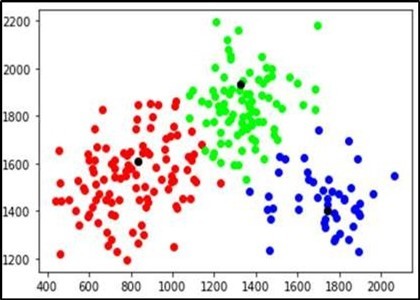
Runtime
Execution time has been measured by the required time for forming clusters by the clustering algorithms k- means, PAM and CLARANS. Time required for each algorithm has been recorded and results have been drawn. Computing time (in seconds) are shown in table 1 and table 2. For this work we choose two spatial datasets (312 data) and flame (240 data). A graphical representation of results has been created in Figure 12 and Figure 13, which is a chart used for comparison with clustering algorithms.
Figure 12.Time chart of k-means, PAM and CLARANS algorithms to form three clusters of different dataset.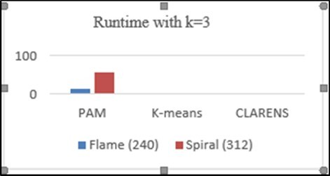
Figure 13.Time chart of k-means, PAM and CLARANS algorithms to form ten clusters of different dataset.
| Dataset | PAM | Kmeans | CLARANS |
| Flame (240) | 13.8 | 0.5 | 0.21 |
| Spiral (312) | 56.4 | 1.69 | 0.36 |
| Dataset | PAM | Kmeans | CLARANS |
| Flame (240) | 363.63 | 3.34 | 0.6 |
| Spiral (312) | 304.53 | 6.11 | 0.68 |
Comparing computing time of the clustering algorithms hows that the CLARANS algorithm takes less time than others, that means this work indicates CLARANS performance is better than others according to time chart.
All the proposed algorithms has been implemented using programming language python. From the experimental results, the graphical representation shows that CLARANS has a low execution time value compared to other algorithms for (k = 3 (0.21; 0.36)), (k = 10 (0.60; 0.68)) even if we have to change the value of k, and also the size of dataset but PAM has a longer execution time.
for the execution time of Kmeans has an intermediate value between the two algorithms.
the number of k clusters has an influence on the execution time.
the size of dataset has an effect on the variation of the execution time. Clarans is the best clustering algorithm compared to PAM and K-MEANS.
Conclusion
Clustering is an unsupervised method aimed at grouping and creating a collection of similar objects within the same group . . This work is about algorithms of clustering and their effectiveness for spatial data mining. The experimental result indicates that CLARANS algorithm reduces the execution time and gives better clusters when compared with other algorithms. But it’s not always the case. CLARANS doesn’t give better cluster. So future research work will be first focused on developing an algorithm, which will increase the performance of segmentation process. Further work also lies in this area. A result line can be drawn from this experimental work and is it is that CLARANS algorithm has better efficiency than PAM and K-MEANS algorithm.
References
- 1.Ch.N.Santhosh Kumar.(2012).Spatial Data Mining using Cluster Analysis. , International Journal of Computer Science & Information Technology (IJCSIT) Vol 4(4).
- 2.Aksac Alper.Tansel Ozyer and Reda Alhajj, (2020).Data on cut-edge for spatial clustering based onproximity graphs,ElsevierDatain brief28.
- 3.Liu Yaohui, Liu Dong, Yu Fang, Ma Zhengming. (2020) A Double-Density Clustering Method Basedon “Nearest to First in”Strategy,Symmetry. 12-747.
- 5.Mark J Embrechts, Christopher J Gatti, Linton Jonathan, Roysam Badrinath. (2013) Hierarchical Clustering for Large Data Sets, in book:AdvancesinIntelligent SignalProcessingandDataMining.
- 6.J H Ward. (1963) Hierarchical grouping to optimise an objective function. , Journal of the American Statistic Association 58, 236-244.
- 8.Fakir Youssef, Elklil Jihane. (2021) Clustering Techniques for Big Data Mining. Lecture Notes in Business Information Processing book series(LNBIP 416.
- 9.J B MacQueen. (1967) Some methods for classification and analysis of multivariate observations. inProceedings of the 5thBerkeley SymposiumonMathematicalStatisticsandProbability,Vol 1, 281-297.
- 10.A P Reynolds, Richards G, V J Rayward-Smith. (2004) The application of K-medoids and PAM to the clustering of rules. in Proceedings of theFifth International Conference on IntelligentData EngineeringandAutomatedLearning (IDEAL’04) in Z. R. Yang, H. Yin, and R. Everson (eds.) 173-178.